Statistics and Probability Basics
Published:
Law of Large Numbers
In a nutshell, the Law of Large Numbers says that when we take a large number of independent samples from a distribution, the mean of the samples drawn is very close to the mean of the distribution.
To state the law, let’s say we have drawn \( n \) independent and identically distributed (i.i.d) samples \({X_1, X_2, …, X_n}\) from a distribution with mean \( \mu \) and variance \( \sigma^2 \). Note: this only works if the distribution has a mean and a variance.
Now, given the samples, we can define the sample mean \( \bar{X_n} \) as:
\[\bar{X_n} = \frac{1}{n} \sum_{i=1}^{n} X_i\]The Law of Large Numbers says that as \( n \) grows, the sample mean \( \bar{X_n} \) converges to the true mean \( \mu \). This is important because while we can calculate the mean of theoretical distributions, if we want to verify or figure out the mean of a distribution in the real world, we need to understand the relationship between the sample mean and the mean of the distribution from which the samples are drawn.
It is important to make the distinction that \( \bar{X_n} \) is a random variable because it is made as a sum of random variables, while \( \mu \) is a real number. So, what does it mean for a random variable to be close to a real number? In exact terms, it is stated in two ways that are similar but have some important differences.


Weak Law of Large Numbers
The weak law states that for any \( \epsilon > 0, P(\vert \bar{X_n} – \mu \vert > \epsilon) \rightarrow 0 \) as \( n \rightarrow \infty \).
Chebyshev’s inequality says that for any random variable X with mean \( \mu \) and variance \( \sigma^2 \), and any real number \( k > 0 \)
\[P(\vert X – \mu \vert \geq k \sigma) \leq \frac{1}{k^2}\]In our case, X is \( \bar{X_n} \), so its mean is \( \mu \) and variance is \( \frac{1}{n^2} (n \sigma^2) = \frac{\sigma^2}{n} \)
Thus, the \(k\) in Chebyshev’s inequality becomes \( \frac{\epsilon \sqrt{n}}{\sigma} \). So we get the inequality
\[P(\vert \bar{X_n} – \mu \vert > \epsilon) \leq \frac{\sigma^2}{n \epsilon^2}\]The RHS, for a constant \( \epsilon \) goes to zero as \( n \) goes to infinity, thus proving the Weak Law of Large Numbers.
Strong law of large numbers
The SLLN states that as n grows to infinity, the sequence \( \bar{X_n} \) converges to \( \mu \) with probability 1. So, if we consider an event where we sequentially draw an infinite number of samples from the distribution, in that event, the probability that the sequence converges to \( \mu \) is 1.
This doesn’t mean that it is impossible for the series to not converge to \( \mu \). For example, if we toss a fair coin and count the number of heads, the ratio of head to total tosses should converge to 0.5 as we make more and more tosses but mathematically speaking there is nothing stopping the coin from landing heads every time and the ratio to be 1, but the probability of that happening keeps getting lower and lower with more tosses and in the limiting case it becomes 0, even though this event is not impossible.
The proof is a little bit more involved this time, you can find it in this paper by N. Etemadi.
Central limit theorem
The Central Limit Theorem is one of the most consequential theorems in statistics and machine learning. The basic result is that when we draw a large number of i.i.d points from a distribution, the sum, or equivalently the mean, of those samples would have a Normal distribution.
Let’s look at \( \bar{X_n} \) again
\[\bar{X_n} = \frac{1}{n} \sum_{i=1}^{n} X_i\]Ignoring the \( 1/n \) scaling term, the remaining part is a sum of i.i.d samples of the distribution, so the expectation of this sum is just the sum of expectations, where the expected value of each term is \( \mu \).
Thus,
\[\mathbb{E}(\bar{X_n}) = (\frac{1}{n})(n \mu) = \mu\] \[\mathbb{E}(\bar{X_n} - \mu) = 0\]For the variance we get
\[var(\bar{X_n} - \mu) = var(\bar{X_n}) + 0\] \[= \frac{1}{n^2} var(\sum_{i=1}^{n} X_i)\] \[= \frac{1}{n^2} \cdot n \cdot var(X_i)\] \[= \frac{\sigma^2}{n}\]We can scale the term and get
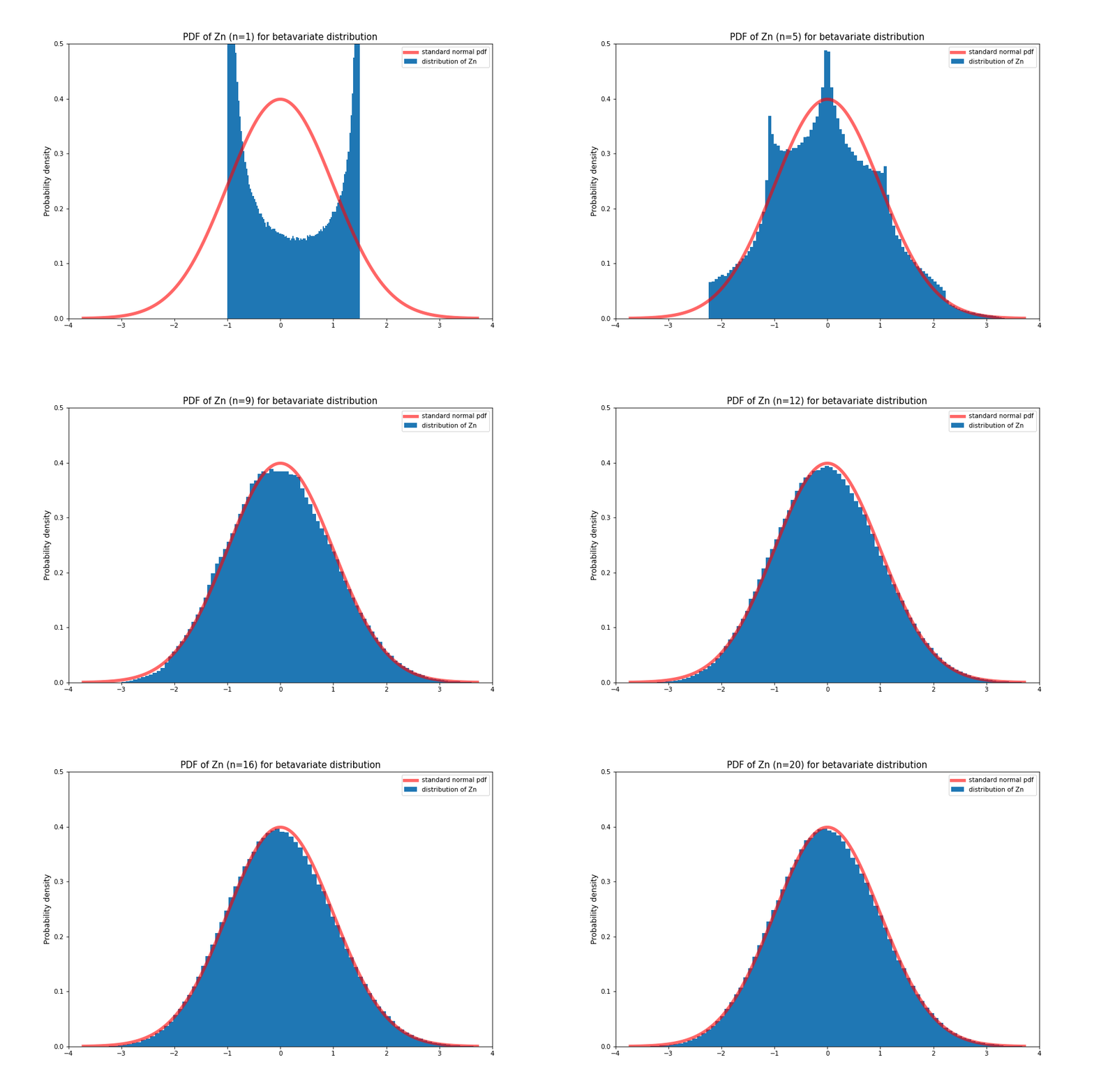
\[Z_n = \frac{\sqrt{n} (\bar{X_n} - \mu)}{\sigma}\]which has 0 mean and unit variance
The central limit theorem says that the distribution of this random variable converges to \( \mathcal{N}(0, 1) \) as \( n \rightarrow \infty \)
The proof of the theorem can be found here.

This is a very important result since it means that even if we don’t know the underlying distribution of some phenomenon, we can approximate the sum of its samples to be gaussian. In most settings, we can assume random noise to be gaussian which makes analyzing its impact much easier.
It also gives us an idea of how fast the sample mean converges to the true mean. Since the term written above has a \( \sqrt{n} \)term in it that keeps it from collapsing to zero or exploding to infinity, it means that regardless of the distribution, the difference between sample mean and true mean will fall to zero at the rate of \( \frac{1}{\sqrt{n}} \).


Leave a Comment