GAN Implementation
Published:
Introduction
GANs or Generative Adversarial Networks are generative models that try to learn the distribution of a given dataset using two neural networks that work against each other while training. You can learn more about them here.
Dataset
In this example we will use the Rock Paper Scissors dataset. This dataset contains about 2500 RGB CGI images of hands in the “stone”, “paper” or “scissors” positions with a 300x300 pixel resolution. Some example images are shown below:


Image resizing
To achieve good performance with such a small dataset and limited compute power, it would be a good idea to make the images grayscale and resize them to a more manageable resolution (for instance 100x100). But I wanted to see how far can we push this method with limited dataset sizes so I used the original size images.
Model
As explained above, the model consists of two neural networks, which are called the generator and the discriminator. The generator tries to generate new points that hopefully look like they were drawn from the original dataset, while the discriminator tries to distinguish between the real data points and the fake ones created by the generator.
Discriminator
This one is relatively simple. Given a bunch of images, it needs to identify which ones are from the original dataset and which ones were created by the generator, i.e., this is a binary classification model. It takes images of size 300x300x3 and produces a single scalar output which is the model’s prediction of whether the given image is real or fake (crated by generator).
In our case, the model is a pretty standard CNN, with a bunch of 2D convolutional and max-pooling layers with leaky-ReLU activation and dropout layers for regularization.
Generator
The generator is in some sense the mirror image of the discriminator. To create a new image, the model needs a random ‘noise’ vector. This noise vector acts as a random seed for the generator. From there, there are a bunch of 2D transpose-convolutional layers with leaky-ReLU activation and batch-normalization until we end up with an image of the same resolution as the training dataset. Hopefully, the contents of the dataset are also reflected in the images created by our generator.
Steps
The code for training the model is adapted from the TensorFlow blog on DCGAN.
Loss
To start the training process, we need to define the loss functions for both the generator and the discriminator.
For the generator, we want the images generated by it to appear real to the discriminator, thus we want the prediction for the generated images from the discriminator to be close to 1. So, if the prediction by the generator is pred, we can set the loss as:
Lgen = cross_entropy(1, pred)
For the discriminator, we want it to correctly predict the real and fake images. Thus, the loss becomes:
Ldisc = cross_entropy(target, pred);
where,
target = 1 if image is real
target = 0 if image is fake
We sum up the losses for all the images in the batch to get the batch loss.
Optimizer
For both the generator and the discriminator, we use separate instances of the Adam optimizer.
Train step
One train step involves two parts:
- Create a batch of images using the generator and randomly created noise vectors, and get the predictions for them using the discriminator. Calculate the loss for the generator and update the weights of the generator while keeping the weights of the discriminator constant.
- Get a batch of images from the dataset and get the predictions for them using the discriminator. Use both the predictions on the real and the fake images to calculate the loss for the discriminator. Update the weights for the discriminator while keeping the generator weights constant.
The python code for this steps looks like this:
def train(dataset, epochs):

    for epoch in range(epochs):
        start = time.time()
        num_steps_per_epoch = len(dataset)

        gen_train_fake_output = []
        disc_train_real_output = []
        disc_train_fake_output = []

        # Training generator
        for image_batch in range(num_steps_per_epoch):
            fake_output, gen_loss = train_gen()
            gen_train_fake_output.append(fake_output)

        # Training discriminator
        for image_batch in dataset.take(num_steps_per_epoch-1):
            real_output, fake_output, disc_loss = train_disc(image_batch)
            disc_train_real_output.append(real_output)
            disc_train_fake_output.append(fake_output)
Repeating these for multiple passes over the dataset should hopefully teach the generator what the images in the original dataset look like through the predictions made by the discriminator.
Results
The model starts showing acceptable results after about 100 epochs of training. If we look at the results after each epoch we can see that during the training process the generator starts by creating the basic outline of a hand and the adds more details as the training continues.

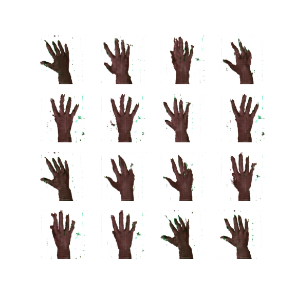
Training a GAN can be a little tricky, and the process can easily collapse giving meaningless results. After a few tries, I got these results from my model:

The results show images that resemble the general shape of the hands in the ‘paper’ or ‘scissors’ shape (getting ‘rock’ images is rare), but lack detail. While these images are nowhere near photorealistic, they look pretty good considering the amount of data and computing power used to train the model.
Different architectures for the generator and discriminator might also improve the results, the architecture I used was something I randomly created without putting a lot of effort in finding the best hyperparameters.
How well the GAN performs depends on the initial conditions, so training the model twice with the same config but different random seeds can give very different results.
Possible improvements
Many techniques can be applied to improve the model performance like:
- Increasing the size of the dataset - by data augmentation or generating more data points (which is possible in this case since the images are created by CGI)
- Progressively growing the size of the images during training. See StyleGAN 2
- Using different loss functions

