Introduction

Naive Bayes is a text classifier that uses Bayes’ rule along with a few simplifying assumptions to predict the class of an unseen document.

For a classification task, we are given a document \(D\) and need to predict the class \(c \in C\) where \(C\) is the set of possible classes. To do this, we calculate the probability of the predicted class given the document \(P(c|D)\). The class with the highest posterior probability is our predicted class.

Using Bayes’ rule we can write

Now, we apply the naive assumptions of Naive Bayes, which are the following-

1. The order of words in a sentence is not important, so we can use a bag-of-words model.
2. Occurrence of words is conditionally independent given a class in a document, i.e., there is no correlation between occurrence of different words for a given class.

Using these two assumptions, we can define our predicted class as-

Where \(w_i\) are the words in the document \(D\).

To avoid numerical instability that might arise due to multiplying a lot of small numbers together, we can take the logarithm of the posterior probabilities. Thus-

Dataset

For this project, we will use the Coronavirus tweets text classification model from Kaggle. The dataset contains tweets related to COVID-19 and the sentiment of the tweet belonging to one of the five classes- “Extremely Negative”, “Negative”, “Neutral”, “Positive”, “Extremely Positive”.

There are about 41k rows in the training set and about 3.8k rows in the test set, which have been separated for us by the authors of the dataset.

Preprocessing

The tweets in the dataset are unprocessed and we need to clean the data a bit before we can begin training our model.

Since we only want to make predictions based on the words in the tweet, we will remove any non-ascii characters, usernames, URLs, punctuations, and numbers. We will also convert all the words to lowercase so that “banana” and “Banana” are not considered different words.

The preprocessing function performs all these steps sequentially.

def preprocess(sentence:str)->str:
    # Remove non-ascii characters
    sentence = ''.join([i if ord(i) < 128 else '' for i in sentence])

    # Remove @usernames
    sentence = re.sub('@[^\s]+ ?','',sentence)

    # Remove URLs
    sentence = re. sub(r'\S*https?:\S*', '', sentence)

    # Remove punctuations
    sentence = re.sub('[^\w\s]', ' ', sentence)
    sentence = re.sub('_', ' ', sentence)

    # Remove \n and \r
    sentence = re.sub('\\r', '', sentence)
    sentence = re.sub('\\n', '', sentence)

    # Remove numbers
    sentence = re.sub('[0-9]+', '', sentence)

    # Replace multiple spaces with single space
    sentence = re.sub(' +', ' ', sentence)

    # Convert to lowercase
    sentence = sentence.lower()

    return sentence.rstrip()

We will also need to convert classes from text to numerical form. If we want, we can also convert the problem into a binary classification problem. For example, we can consider every tweet “Neutral” and above as positive, while “Negative” and “Extremely Negative” tweets can be considered negative.

Creating the vocabulary

Once we have cleaned the data, we can use the preprocessed tweets to build our vocabulary, which is a set of all words that our model recognizes. In our case, we find that after preprocessing, our training set has 45,605 different words, but a large number of them might only be used a few times, like someone’s name, a typo, etc.

Vocab = dict()
for idx, row in train_df.iterrows():
    sentence = row['text']
    for word in sentence.split(' '):
        Vocab[word] = Vocab.get(word, 0) + 1

Thus, to only keep commonly used words, we remove any words that occur fewer times than a threshold (10 in our case).

# Removing uncommon words
num_threshold = config['training']['word_count_threshold']
words = list(Vocab.keys())
for word in words:
    if Vocab[word] < num_threshold:
        del Vocab[word]

This brings our vocabulary size from 45,605 down to only 6,778 - a much more manageable number for a dataset of the size we have.

Calculating class-wise probabilities

Once we have our vocabulary, we can calculate the class-wise word probabilities, which is the number of times a word occurs with a given class divided by the total number of words that occur in that class. We can use Laplace Smoothing to make sure that words don’t get assigned probabilities of 0, which cannot be conditioned away. Thus, we can calculate the class-wise probabilities as-

To access the conditional probability of a word, we will also build data structures that will map words to their indices in the probability table and vice-versa.

Predicting the class

Once we have the class-wise probabilities, we can use them combined with the prior probabilities of different classes, which is just the fraction of times each class is present in the training set, to predict the document class.

For each class, we take the words in the given document. If a word is part of our vocabulary, we look up its conditional probability from the table we just computed and use it to calculate the log posterior probability of the class. Any words that are not in our vocabulary are discarded as if they were not in the sentence at all.

Finally, we call the class with the highest log posterior probability our predicted class.

Measuring performance

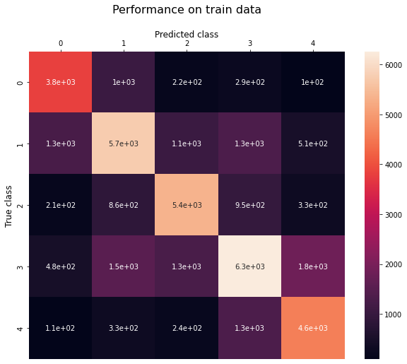
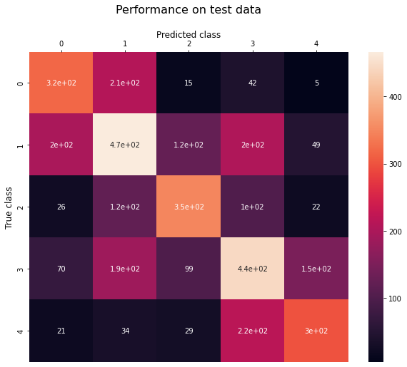
Once trained, we can measure how well our model performs on the training and test sets by looking at metrics such as accuracy, precision, recall, and F1-score. We can also look at the confusion matrix where the rows represent the true classes and the columns represent the predicted classes.

Performance on training data

The confusion matrix for the training data is as follows-

And the other performance metrics are-

1. Accuracy: 62.711%
2. Precision: 62.964%
3. Recall: 64.353%
4. F1-Score: 63.545%

Performance on test data

The confusion matrix for the test data is as follows-

And the other performance metrics are-

1. Accuracy: 49.421%
2. Precision: 50.793%
3. Recall: 50.379%
4. F1-Score: 50.516%

We can see our model does not perform as well on the test data as it did on the training set. This is to be expected since all models overfit a little bit on their training data. Still, we get pretty decent results considering that this is a 5-class classification problem with a relatively small training set.

Looking at the confusion matrix we can also see that most of the mistakes are “close” to the correct answer, and the model rarely misclassifies “Extremely Negative” tweets as “Extremely Positive” or vice-versa.

Generating new sentences

Since we have calculated the conditional probabilities of different words, we can use them to sample words and create new sentences. Some examples for different classes are-

1. Extremely Negative

   for be that sky make slot to coronavirus

   ban people on panic protective amazon a

2. Negative

   at due that california financial of the new

   service with a disruptions had delay with people

3. Neutral

   covid to wfh to food up to our

   brussels situation prices founder said on to quarantinediaries

4. Positive

   and behaviour this also two amid how life

   and s are printing policy of if clothes

5. Extremely Positive

   jan help of please customers cheap deserve learn

   you online delivery of have through toiletpapergate s

We can see that the sentences don’t make a lot of grammatical sense, which is to be expected since our model never learns any sense of word order. Still, we can see which words the model considers important while making classification.

Conclusion

As we can see, Naive Bayes is a very simple yet robust model for text classification that works well especially in cases where the data is limited.

It can be used as a baseline to compare performance of other, more complex classification models.

References

1. Playlist - Week 2: Naive Bayes, Text Classification, and Sentiment | From Languages to Information | YouTube
2. Bag-of-words model - Wikipedia
3. Coronavirus tweets NLP - Text Classification | Kaggle
4. Laplace smoothing in Naïve Bayes algorithm | Towards Data Science